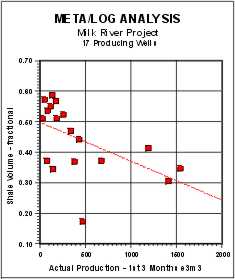
Average shale volume was correlated with actual production but the correlation coefficient was only 0.296, although the trend of the data is quite clear.
This amplifies the shale indicator in cleaner zones and is scaled the same as the GR curve. A net reservoir cutoff of Qual2 <= 50 on this curve was a rough indicator of first three months production, but the correlation coefficient was as poor as for average shale volume. QUAL2 does make a useful curve on a depth plot as it shows the best places to perforate when density and neutron data are missing.
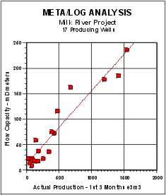
This graph is converted to a numerical quality indicator (Qual1) in a complex series of equations that represents predicted flow rate. The
equations, as displayed in the Lotus 1-2-3 spreadsheet are as
follows: Where:
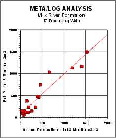
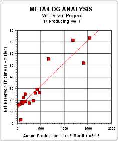
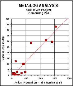
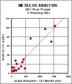
Note that these nested IF statements are slightly different than those originally published by Hester. The changes correct for typographical errors in the original paper. There is a flaw in Hester’s paper that can be cured. He does not account for zone thickness or attempt to find a net reservoir number. He uses only the average quality number over the zone, which presupposes that all perforated intervals are equal in thickness. To overcome this, we can use a quality cutoff and obtain a thickness weighted quality and correlate this to actual production. A Hester quality of 4.0 or higher reflects reservoir rock that is worth perforating, and gives similar net reservoir thickness as the previous indicators. Graphs showing the correlation of actual production to net reservoir with QUAL1 >=5 and >=4 are shown below. The regression coefficients are 0.856 and 0.837 respectively. Although this looks pretty good, the low rate data is clustered very badly and other indicators work better in low rate wells. The Hester quality number QUAL1, along with QUAL2 = GR / RESD, are the only quality indicators that show where to perforate. The other indicators described here give a reasonable estimate of reservoir performance, but do not give any indication of how to economically complete the well.
The leading constant takes into account borehole radius, drainage radius, viscosity, and units conversions. KH is flow capacity in md-meters. (PF - PS) is the difference between formation pressure and surface pressure in KPa. A constant value of 1300 KPa was assumed for this study. Clearly, more detailed data could be used if time permits. TF was chosen constant at 20 degrees Celsius. FR is a hydraulic fracture multiplier, chosen as 2.0 for this study, based on the 9 wells used to calibrate to 3-month initial production data. The constant 90 converts e3m3/day into an estimated 3-month production for comparison to actual. The 3 month numbers were chosen instead of daily rate as they have more “heft” and can be equated to income more readily. Note that the equation used is a constant scaling of KH, so the correlation coefficient is the same as the KH graph at 0.906.
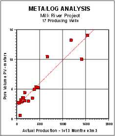
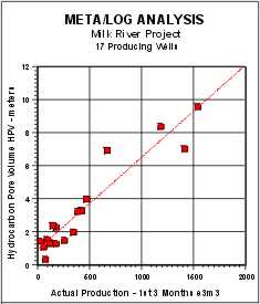
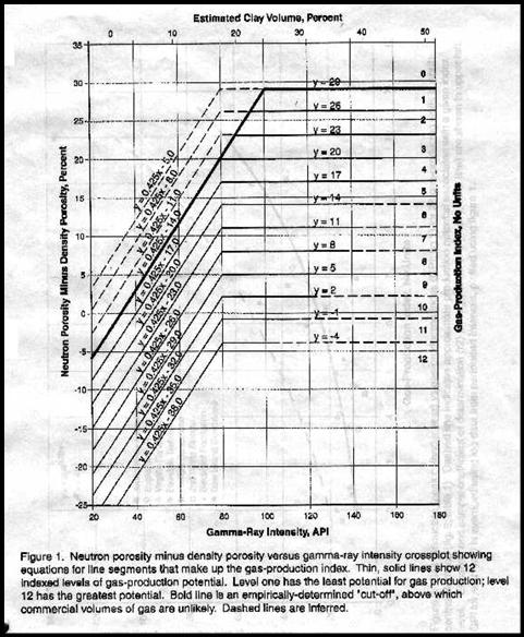
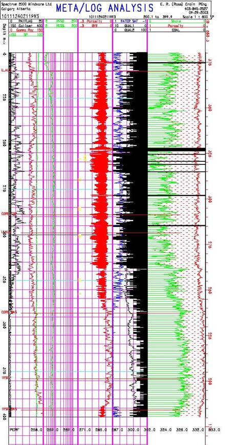
The conventional analysis, plotted in Track 5, gives a clear picture of why the conventional approach is so discouraging. Unfortunately, the laminated models do not create output curves that are consistent with a depth plot, so it is impossible to make pretty pictures of the results except in map form. In the current Milk River study, this model appears to be the most effective in predicting reasonable reservoir properties. PHIMAX was set at 0.20, based on core data, and KBUCKL was set at 0.040, based on experience. CPERM and DPERM were chosen as 18.3 and -3.00 respectively from the core data crossplot shown earlier. A total of 10 reservoir quality indicators for each of 3 reservoir layers, plus the cored interval and the perforated interval were generated for each of 4 different analysis models. The best model for predicting productivity is Model C, using the minimum of 3 shale indicators. The density neutron porosity separation indicator is essential to the success of Model C. The best productivity indicator is the flow capacity (KH) or its equivalent productivity estimate in e3m3 for 90 days (1st 3 months production estimate). Five other indicators have strong correlations with productivity (Net Reservoir, PV, HPV, Hester’s QUAL1 >=5, and QUAL1 >=4). Hester’s number does not have much resolution at low flow rates, but clearly separates poor from good wells. An important use of the summary tables is to determine whether a well is under-achieving due to limited perforation interval or a poor frac job. A comparison of the total KH for the Milk River compared to the KH for the perforated interval will point out any problem wells. Even if KH is badly mis-calibrated, the comparison is useful. Over-achievers may be producing commingled, intentionally or otherwise, from deeper horizons or may point to log data or analytical difficulties.
The models can be used to generate a perforation list from Hester’s quality number or from VSH minimum. An acceptance/rejection filter on the list will shorten it considerably. This will eliminate intervals that are too thin to bother with and group intervals that are close enough to be considered as single intervals. Because
a full log suite was available in the 9 wells used for calibration,
we have obtained the most likely shale volume (Vsh) result. The
8 wells held in reserve to test the model also showed very good
agreement with initial production. One well that calculated an
IP higher than actual can be brought into line with a small tune-up
of the shale density parameter
for initial production comparison |
|
||||||||||||||
|
Page Views ---- Since 01 Jan 2015
Copyright 2023 by Accessible Petrophysics Ltd. CPH Logo, "CPH", "CPH Gold Member", "CPH Platinum Member", "Crain's Rules", "Meta/Log", "Computer-Ready-Math", "Petro/Fusion Scripts" are Trademarks of the Author |
|||||||||||||||

|
||
| Site Navigation | CASE HISTORY LAMINATED SHALY SAND GAS MILK RIVER NIOBRARA | Quick Links |