|
 DENSITY LOG BASICS
This page describes density logs
profiles, in the order of their appearance over the years.
This presentation style provides insights into tool
evolution, and a specific tool’s capabilities and
limitations. You will find most these tool types in your
well files – here’s your chance to learn more about them.
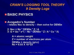
Density logs first appeared in 1957, based on the principle of gamma
ray absorption by Compton scattering.
Early tools were called gamma - gamma density logs because they
emitted and recorded gamma rays. The log displayed counts per
second, which was transformed to density by a semi-logarithmic
transform. Modern tools have two detectors, which allows borehole
compensation to be applied.
They are scaled in units of density
(grams / cc or Kilograms / cubic meter). Some density logs also
record photoelectric capture cross section which is useful in
lithology analysis. Some density logs are displayed in porosity
units (percent or decimal fraction).
The gamma ray source foe all tools is cesium 137.
For more detail on the physics of the density log
measurement, see
Density Theory.
The
tool can be used in air or mud filled open boreholes. A cased
hole tool is available in some areas.
References:
1. Logging Empty Holes
C.G. Rodermund, R.P. Alger, J. Tittman,
Oil and Gas Journal, 1961
2. Formation Density Log Application in Liquid-Filled Holes
R.P. Alger, L.L. Raymer, W.R. Hoyle , M.P. Tixier, JPT, 1964
3. Litho-Density Log Interpretation
J.S. Gardner, J.L. Dumanoir,
SPWLA, 1980
UNCOMPENSATED DENSITY LOG
Early density
logs run by the major service companies had only one detector and were recorded in counts per
second. There were no automatic borehole corrections as there is
today and calibration to density or porosity took some effort.
Such logs are still in widespread use in mineral
exploration and resource assessment. The USGS, NRC, and a number of
independent service companies run slim hole density logs of this design.
I ran a set on Melville Island in the Canadian Arctic in 1969
for sulphur exploration. Aside from trying to stay warm and keep
the liquid ink recorder from freezing up, everything ran
smoothly
for 4 months before returning to gentler climates.
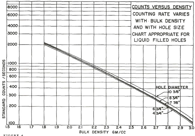
Density is derived with a semi-logarithmic transform. If no
appropriate tool specific chart is available the High Low
porosity technique as described for the neutron log is used.
Here, high count rate = low density = high porosity. Semi-log crossplots of
count rate versus core density or core porosity will calibrate the
method. These tools have a single detector and are not compensated
for borehole effects. Slim hole versions were widely used in strat
holes and in mineral exploration projects. Charts for some specific
tools can be found in the literature, such as the one shown below.
The uncompensated density log produces a single log curve scaled
in counts per second. Some independent logging contractors can
provide a log scaled in porosity or density units. Some
tools were run with a gamma ray log.
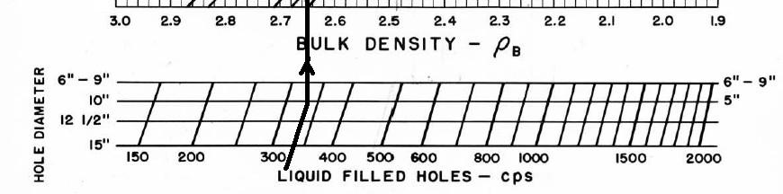
Counts per second to density transform for a Schlumberger PGT-A
density tool. Each tool iteration and each service company requires
a specific chart. Density varies with hole size, mud weight, and mud
cake thickness.
Single detector
density tools are severely affected by hole size, mud weight, mud cake
thickness, source type and strength, source detector spacing, and
detector efficiency. The High-Low calibration method compensates for
all these problems, but available charts do not. In the earliest
versions of these tools, the source strength decayed rapidly, so
count rates definitely need to be normalized on a well by well
basis.
Most density transforms never made it into
published chart books. This one did -
Schlumberger PGT-C or D density count rates to porosity. Additional
charts are available to correct for mud cake thickness and mud
weight, and for air-filled holes. The count rate charts appeared in
1966 chart books, well after they were no longer needed, and
disappeared after 1968. Most density count rate charts are very hard
to find unless you have a good supply of ancient chart books from
1958 through 1968 - a 10 CD set of ancient chart books was
COMPENSATED DENSITY LOG (FDC)
The
borehole compensated formation density logging tool emits gamma rays from a chemical source at the
bottom of the tool The gamma rays enter the surrounding
rocks where some are absorbed. Some gamma rays survive to reach
scintillation counters mounted about 18 and 24 inches above the
source. The number of gamma rays arriving at the far detector is
inversely proportional to the electron density of the rock, which in
turn is proportional to the actual rock density. Data from the
closer detector is used to correct for borehole effects.
Porosity
can be derived from density and can be presented as a percent or as
a decimal fraction on the log. This porosity may still contain
artifacts from shale and minerals not accounted for by the logging
computer, so this porosity is NOT a final answer.
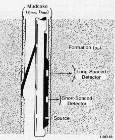 A typical density logging tool is shown
at the right.
The tool is pressed against one side of the borehole by
a back-up arm that also serves to measure a diameter of the
borehole. Two detectors at fixed spacings from the source are
shown. The source is well-shielded from the two detectors and
only scattered gamma radiation is detected. The intensity of
the scattered radiation will be dominated by the density variations
along the path from source to detector. A typical density logging tool is shown
at the right.
The tool is pressed against one side of the borehole by
a back-up arm that also serves to measure a diameter of the
borehole. Two detectors at fixed spacings from the source are
shown. The source is well-shielded from the two detectors and
only scattered gamma radiation is detected. The intensity of
the scattered radiation will be dominated by the density variations
along the path from source to detector.
If there is no stand-off (of mud or mudcake) between the tool face and the formation, and if the
tool is properly calibrated, then the apparent density from
both detectors will be the same and equal to the true formation density.
If they are different, there must be mud between the tool face
and the rock.
If there is some standoff, a correction
to the density from the long spaced detector can be generated
from the difference between the apparent density seen by the
far and the near detectors. The actual correction function
can be determined empirically by placing the density device
in a number of formations to measure the apparent long-spaced
and short-spaced densities for various thicknesses of mudcake
of a variety of densities. Computer modeling has augmented
these laboratory studies.
In addition
to the density and optional porosity curves, a caliper and gamma
ray curve are also presented, along with the density correction
curve. Note that the correction has already been applied to the
recorded density data by the computer in the logging truck.
LITHO-DENSITY LOG (LDT)
The litho density logging tool and
the log display look very similar to the older version, except
for the addition of one new log curve, the photo electric effect
(PE or PEF).
The energy of the returning gamma rays is a function of the PEF
of the rock, which is indicative of mineralogy. To measure PEF,
the detectors were changed to measure both gamma ray count rates
for the density measurement and also the gamma ray energy levels
for the PEF measurement.
Most modern two-detector density devices
use multiple energy windows to derive the density, the photoelectric
factor, and the correction curve. In one
three-detector wireline version, the combination of multiple
detectors and multiple energy windows produce on the order
of a dozen counting rate measurements at each depth. Each counting rate can be described
by a forward model relating the rate to the five important
parameters of density logging: formation density, formation
photoelectric factor, mudcake density, mudcake photoelectric
factor, and the thickness of the mudcake.
For more detail on the physics of the
PEF measurement, see
Density Theory.
The log curves presented are the same as the older FDC log, with
the PEF added.
ADVERSE BOREHOLE CONDITIONS
Standoff caused by rough or large borehole leads to useless
density data if the problem is severe enough. The density correction
curve, the caliper curve, and the density curve itself help to flag
these intervals. Because the backup arm exerts considerable
pressure, mudcake thickness is not usually an issue, but that same
pressure forces the measuring skid into the large diameter of an
oval borehole. This occurs in stressed regions. The large diameter
has the worst borehole condition so we get the worst possible
density log.
In the mid 1970's a 90 degree offset tool was developed to
reduce the chance of logging the large diameter of the borehole. It
consisted of a second backup arm at 90 degrees to the original,
pressured a little higher, that forced the tool skid into the
smaller diameter. This led to the concept of the dual axis, or X and
Y axis calipers. Later development led to a dual density tool,
essentially two complete density logs on the same tool string,
positioned at 90 degrees from each other, resulting in reasonable
complete log coverage in stressed boreholes.
CAUTION: Do not use density data when you suspect standoff
problems. A reasonable guide would be a density correction more than
0.15 gm/cc (150 kg/m3) is highly suspect and greater than 0.20 gm/cc
is useless. If density porosity is greater than neutron porosity,
and no gas is expected in the rock, the density is probably useless
(provided the logs were run on a porosity scale appropriate for the
mineralogy). Noisy, hashy, or impossibly high density porosity
probably indicates a bad log, even when the caliper and correction
curve show no problems. The density skid is about 2 feet long so
there can be significant breakouts within that distance that the
caliper cannot see.
DUAL DENSITY LOG AND 90 DEGREE OFFSET TOOL
Some areas are heavily stressed and stress release
during drilling causes oval boreholes or large breakouts in the
maximum stress axis of the borehole. The skid and backup arm of the
density log often end up in this axis so we end up logging the bad
side of the borehole. Another strong-arm caliper set at 90 degrees
to the density caliper forces the density skid into the
good side of the borehole, resulting in better log quality.
Some operators ran several logging passes in an effort to get the 90
degree offset tool to log most of the interval on the good side of
the hole.
The 90 degree technique is still used but doesn't always succeed.
An alternative was called the dual density
log. There were literally two density tools coupled together, one
above the other at 90 degrees so that while one tool was facing the
bad side of the borehole, the other was facing the good side. Thus
two independent density logs were run simultaneously.
During data processing, the computer code was adapted to take the
maximum of the two density corves, eliminating most of the bad data.
Cable torque forces the tool set to rotate in a stepwise fashion as
it travels up the borehole. There may be minor bad hole effects at
these spots. I am not sure such a combo could be run today.
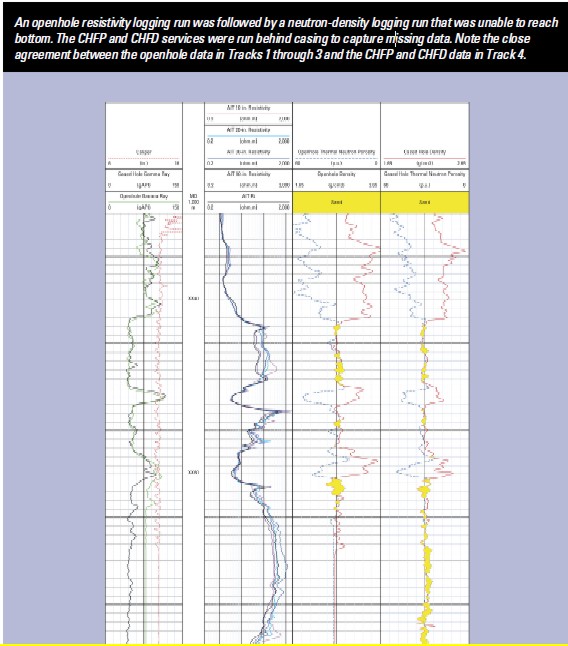
Cased Hole Formation Density (CHFD)
Cased hole formation density logs make accurate formation density
measurements in cased wells. A chemical gamma ray source and
three-detector measurement system are used to make measurements in a
wide range of casing and borehole sizes. The density measurement
made by the three detector system is corrected for casing and cement
thickness.
The
density data are used to calculate porosity and determine the
lithology. The combination of density and neutron data is used to
indicate the presence of gas.
Applications
■ Porosity determination
■ Lithology analysis and identification of minerals
■ Gas detection
■ Hydrocarbon density determination
■ Shaly sand interpretation
■ Rock mechanical properties calculations
■ Determination of overburden pressure
■ Synthetic seismogram for correlation with seismic
DENSITY POROSITY LOGS
Density is proportional to porosity, shale content,
and matrix rock type, just as for the sonic log. Both are also
affected by the fluid in the formation and both must be run
in a liquid filled borehole, although the liquid does not have
to conduct electricity.
Compensated density log presentation
showing density (solid line), density porosity on a
limestone
scale (dashed line), and density correction, plus gamma ray
and caliper in Track 1.
The density log can be presented in units of density,
that is, grams per cc or Kilograms per cubic meter. Some log
presentations portray the density data as its equivalent porosity,
translated with a particular lithology assumption. Some show
both density and density porosity, as in the image above.
The scales are usually called Sandstone or Limestone
scales to reflect the assumption that was made to create them.
Dolomite scales also exist on a few logs. The relationships
are:
1: PHID = (DENS - KD6) / (KD7 - KD6)
2: DENS = PHID * KD7 + (1 - PHID) * KD6
Where:
KD6 = 2.65 for Sandstone scale (English)
KD6 = 2.71 for Limestone scale (English)
KD6 = 2.87 for Dolomite scale (English)
KD6 = 2650 for Sandstone scale (Metric)
KD6 = 2710 for Limestone scale (Metric)
KD6 = 2870 for Dolomite scale (Metric)
KD7 = 1.00 for English units
KD7 = 1000 for Metric units
Because some logs do not have a density scale, you
may have to translate the recorded log into density units so
that it can be used, for example to calculate acoustic impedance
for a seismic application.
To use data from a density log, you must correctly
identify both the scale type, lithology assumption, and the
two end point values. Other log curves are often present, such
as the density correction, compensated neutron, gamma ray,
caliper, bit size, cable tension, and photoelectric effect. You have to choose the correct curve from
among those presented. Editing for bad hole and casing effects
will be mandatory if the log is to be used to generate a synthetic
seismogram. The density data should not be used for any purpose
if the density correct is larger than 0.200 gm/cc (200 kg/m3).
CAUTION: The use of an inappropriate porosity scale on a
combination density - neutron log presentation can be EXTREMELY
misleading. For example, sandstone rock recorded on a limestone
scale will cause the density porosity to be higher than the neutron
porosity by as much as 6 to 8% (0.06 to 0.08 decimal fraction). This
is often interpreted to indicate the presence of gas, leading to
very expensive completion mistakes. The density - neutron crossover
needs to be considerably greater than 8% to indicate gas in this
situation. Similarly, a log run on dolomite scale through a
limestone rock will show up to 12% porosity crossover, just because
of the inappropriate scale, not because of gas. Use the PE curve to
determine lithology, then interpret the crossover correctly. PE near
2 = sandstone, PE near 3 = dolomite, PE near 5 = limestone.
DENSITY INTERFACE LOG and SONAR LOGS
Storage caverns are created on
purpose in salt beds to store gas or oil near points of demand to
help meet peak loads. They must be tested before use and monitored
during use with specialized logging tools.
Density interface logs are used to look for fluid
interfaces in existing oil or gas storage caverns. Sonar logs are
used to find the distance to the cavern wall in a 360 degee survey
that helps determine the cavern volume. Pressure tests are used to
check cavern an wellbore integrity. 3-D seismic surveys are run
prior to cavern construction to locate faults and fractures aboce
and below a proposed cavern site. 3-D seismic may also be used in
exicting salt solution mines before conversion to hydrocarbon
storage.
You don't need a very sophisticated
or well calibrated density logging tool to do this work. A single detector tool recording
its response in counts per second (cps) will do the job. They can be
run on slick line with a memory device or on wireline in real time.
The logs may be non-standard in presentation and may not be recorded
in digital files in LAS format.
During the initial mechanical interface test
(MIT) of a gas storage cavern, the survey is run in time-lapse mode.
With some water in the cavern, nitrogen is injected under pressure
and held for at least 24 hours. If the water level changes or
pressure drops more than 10 psi,
the test has failed. Remedial action, if possible, must be
undertaken before the cavern can be used to store gas. During
operation of the cavern, the objective is to observe the water--gas
contact depth in the cavern, along with the reservoir pressure, to
monitor remaining gas volume.
The original cavern volume is determined by a
sonar log. This device maps the travel time of sound from the tool
to the cavern wall and back again. By pinging the sonar in varying
directions, a map of the distance to the walls can be made at
various depths in the cavern. The survey ends up as a 3-D image of
the cavern, which is used for routine gas volume modeling.
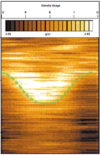 LWD DENSITY IMAGE LOG
Logging while drilling (LWD) offers many alternatives that can be
displayed as an image log. The example at right is a density image
log. Low density values are shaded dark and can be interpreted as
porosity or shale. A gamma ray log run with the drill string helps
distinguish between these alternatives. White colours represent low
porosity or tight rocks.
The LWD density tool is a focused source and detector set, similar
in concept to an open hole density logging tool. As it
rotates, it scans the borehole wall to form the image. Data is
stored in memory downhole, while only the composite density curve is
sent uphole, where it is displayed in standard well log format
along with any other LWD curves available in the tool string.
DENSITY LOG CURVE NAMES
Formation Density Log Uncompensated Type (DL)
| Curves |
Units |
Abbreviations |
| density
count rate |
cps |
DCPS |
| *
gamma ray |
API |
GR |
| *
caliper |
in
or mm |
CAL |
Formation Density Log Compensated Type (FDC)
| Curves |
Units |
Abbreviations |
|
density |
gm/cc
or kg/m3 |
RHOB or DENS |
|
gamma ray |
API |
GR |
| *
porosity from density |
%
or frac |
DPHI
or PHID |
| *
formation factor from density |
frac |
FD |
| caliper |
in
or mm |
CAL |
| *
density correction |
gm/cc
or kg/m3 |
DRHO |
This log was often presented on the same log
display as the compensated neutron log, and more rarely
in the right hand track on a dual induction log.
Litho-Density Log (LDT)
| Curves |
Units |
Abbreviations |
|
density |
gm/cc
or kg/m3 |
RHOB or DENS |
|
gamma ray |
API |
GR |
| *
porosity from density |
%
or frac |
DPHI
or PHID |
| *
formation factor from density |
frac |
FD |
| caliper |
in
or mm |
CAL |
| *
density correction |
gm/cc
or kg/m3 |
DRHO |
| photo
electric cross section |
cu |
PE |
This log was often presented on
the same log display as the compensated neutron log,
EXAMPLES OF DENSITY LOGS
Density logs presented with other log curves - neutron - density
(top right) and induction -
density (bottom left).
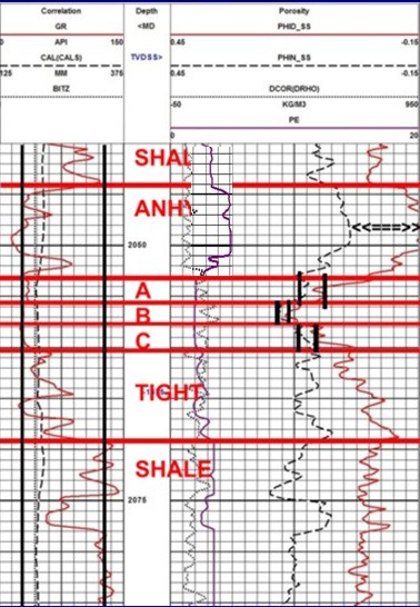
Typical display format for
PE-density porosity-neutron porosity log on a sandstone scale. The
density correction curve may appear on the left or right side of the
wide track. A density scale of 1.65 to 2.65 gm/cc may be used
instead of the density porosity scale.
|